In this exercise we’ll create forecasts for a new product using the Bass diffusion model. The Bass model is most often used to forecast first-time purchases of new-to-world products.
The model tries to capture the adoption rates of two types of users—innovators and imitators. Innovators are early adopters of new products and are driven by their desire to try new technology. Imitators are more wary of new technology—they tend to adopt only after receiving feedback from others.
The Bass model uses two coefficients to quantify the adoption rates. The Coefficient of Innovation, referred to in the literature as “p”, controls the rate for the innovators. The Coefficient of Imitation, referred to in the literature as “q” controls the rate for the imitators.
If you have 5 or more historic data points, these coefficients can be fit to the data. To build a Bass model with fewer than 5 data points you must set the values for these coefficients along with the total number of potential adopters.
In this exercise, we will look at two examples—one where no data are available for the new product and the other where the initial 6 years of adoptions are known.
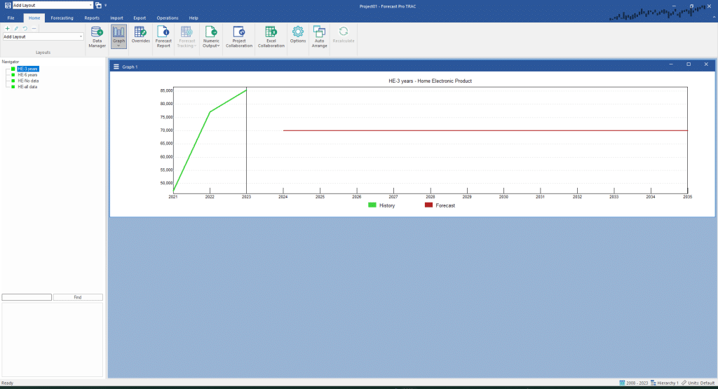
Start the program and click the New Project icon. On the Home tab, open the Data Manager and specify Home Electronic Product.xls on the Historic Data Row. Click the Read & Forecast button and then click Exit to exit the Data Manager. Close the Override view.

Select HE-No data on the Navigator, go to the Forecasting tab and click the Bass Diffusion icon.
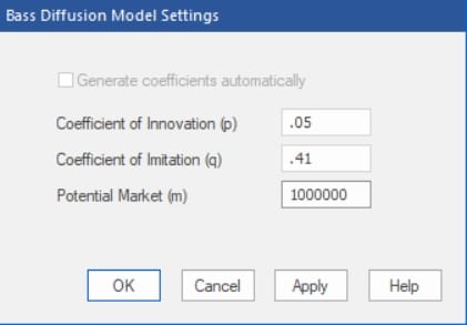
In this example we have no historic data so we will need to specify the Coefficient of Innovation, the Coefficient of Imitation and the Potential Market. The coefficients could be set using values from an analogous product’s model. There is also a considerable body of literature on the Bass model including published coefficients for different types of technology. Consult the Forecast Pro Statistical Reference Manual for details.

The example we are working with is a home electronic device. Our market research suggests the total market is 1 million units. A similar product had coefficients of innovation and imitation of 0.05 and 0.41 respectively. Edit the settings to match the ones above and click OK to build the model.
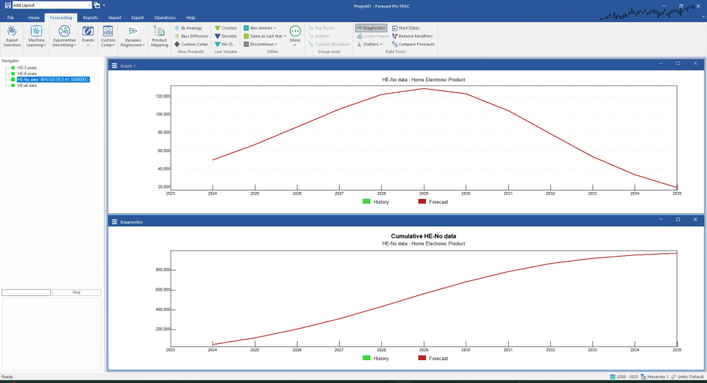
On the Forecasting tab, click the Diagnostics icon in the Tools group (far right) to open the Diagnostics view. Right click the Diagnostics view to invoke its context menu and select Cumulative. Your display should now match the one below.

The top graph shows the forecast of the number of first-time adopters growing for the first five years and then declining. The bottom graph shows the forecast of the number of first-time adopters on a cumulative basis (therefore each period displays total first-time adoptions to date). Notice the cumulative forecasts resemble an elongated “S”. This characteristic shape is why the Bass model is often referred to as an S-curve model.
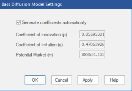
Select HE-6-years on the Navigator and click the Bass Diffusion icon on the Forecasting tab to invoke the dialog box below.

Notice that now that we have more than 5 data points, Forecast Pro can automatically fit the coefficients and estimate the potential market from the data. The estimated coefficients are pretty similar to the ones we used prior to having data, however, the estimate of the potential market is a good bit lower. Click OK to build the model.
Forecasting sales for a new-to-world product prior to launch is extremely difficult. Regardless of the forecasting method used, you should be constantly revisiting your model assumptions as data becomes available and adjusting the model when appropriate.
Exit Forecast Pro.

