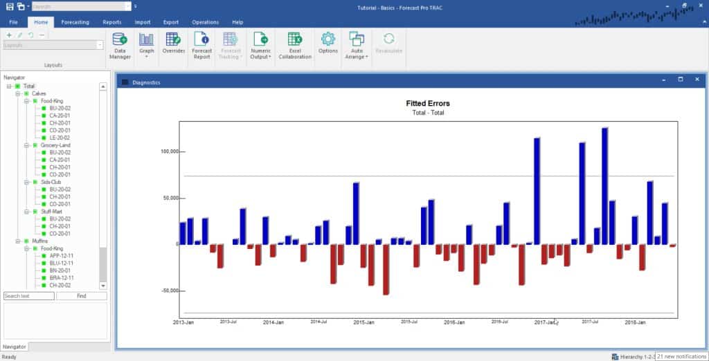
The diagnostics view provides a variety of statistical displays to assist you in building and diagnosing custom models. To open the diagnostics view, click the Diagnostics icon in the Data Tools group on the Forecasting tab or select Diagnostics from the drop-down on the Graph icon on the Home tab or Reports tab.

The default view is the Fitted Errors graph. Use this display to identify outliers or other problem areas of your data. The dashed horizontal lines mark the 2.5 and 97.5 percentiles. About one error in twenty extends beyond these limits.
You can right click on the Fitted Errors graph to bring up the Advanced Diagnostics context menu or use the hamburger menu in the top left of the view and select one of the other available diagnostic graphs.
Error ACF displays a graph of the error autocorrelation function. Use the error ACF to make quick assessments of correlational models like Box-Jenkins and dynamic regression. If your statistical model is well specified, then about one autocorrelation in twenty falls outside the limits marked by dashed lines, and the autocorrelations are not patterned. The computation of the error autocorrelation function is covered in the Forecast Pro Statistical Reference Manual.
ACF and PACF are provided to help you manually identify ARIMA models. The autocorrelation function (ACF) is used to identify differencing, and to identify the number of simple and seasonal MA terms. To identify differencing, select Advanced Diagnostics Settings on the context menu.

Use the Automatic button to display the differencing values selected by Forecast Pro’s automatic Box-Jenkins algorithm. Use the partial autocorrelation functions (PACF) to identify the number of simple and seasonal AR terms. Refer to the Forecast Pro Statistical Reference Manual for further information about manual identification of ARIMA models. The ACF and PACF may also be helpful for manually identifying the dynamic terms in a dynamic regression model.
Cumulative displays a cumulative graph of the currently selected item. This is especially useful when examining a Bass Diffusion model.

