In this first example we will prepare a five-year forecast and experiment with customizing the trend.

Start Forecast Pro and click the New Project icon. The data we will be using is monthly and the first step will be to set the forecast horizon to 60 so that we will generate a 5-year forecast. From the Home tab, select the Options icon to open the Options dialog box shown below.

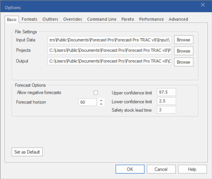
Set the Forecast horizon field to 60 and click OK. Click the Data Manager icon to call up the Data Manager. Click the Add drop-down on the Historic Data row, select Excel and select Telecom installations.xls to add it to the Historic Data row.

Click the Read & Forecast button to read in the historic demand data and generate the statistical forecasts.

Click the Exit button to exit the Data Manager. Close the Override view and click Auto Arrange on the Home tab or the Quick Access Toolbar. Your display should now match the one shown below.

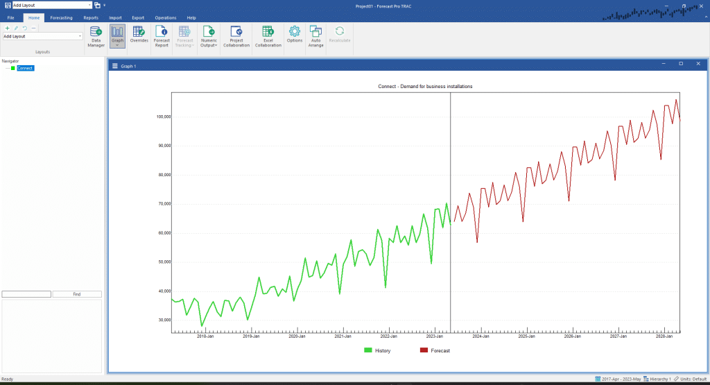
The data represent monthly demand for telephone installations. Notice the data and forecasts exhibit a strong trend and seasonal pattern. Notice also that expert selection chose to forecast this data set using a Box-Jenkins model.

Select the Forecasting tab. Notice that there is a large Custom Component icon and a small icon in the New Products group. Click either icon to invoke the Component Model Settings dialog box. Click the Apply button to build the initial model. Move the Component Model Settings dialog box so that you can clearly see the graph. Your screen should now match the one below.

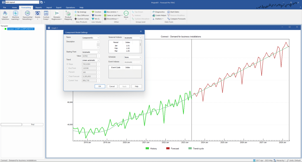
The initial model automatically calculates each component using an exponential smoothing approach. Notice that the Starting Point is currently set to Automatic and has a value of 65782. The Trend is set to linear automatic and has a slope of 742 units per month. The Seasonal Indexes are set to Automatic and are displayed in the dialog box. We have not defined an event schedule, so Event Indexes are not used.

The green line running through the history and forecasts on the graph is the trend component. As noted above the automatic approach yields a linear (straight line) trend that increases 742 units a month for the next 5 years.

This is a very aggressive long-term forecast. Let’s say that our knowledge of the market leads us to believe that this kind of growth is unlikely to be maintained and we therefore wish to modify the underlying trend component of the forecast.

Open the Trend drop-down. Notice there are three types of trends supported (None, Linear, Bent) and that the linear and bent types have both an automatic and custom option. Choose Linear custom.

Linear custom will use a linear trend but allow you to control the slope. You can use the Slope option to set the slope directly or use the End Point, Total Forecast or Current Year options to have Forecast Pro calculate the new slope.

Set the Total Forecast field to 4,500,000 and click the Apply button.

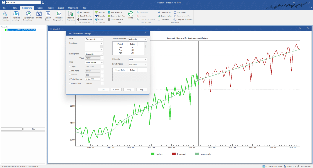
Notice the forecast now reflects the new slope (302 units per month) and the values for the End Point, Total Forecast or Current Year options have been updated accordingly.

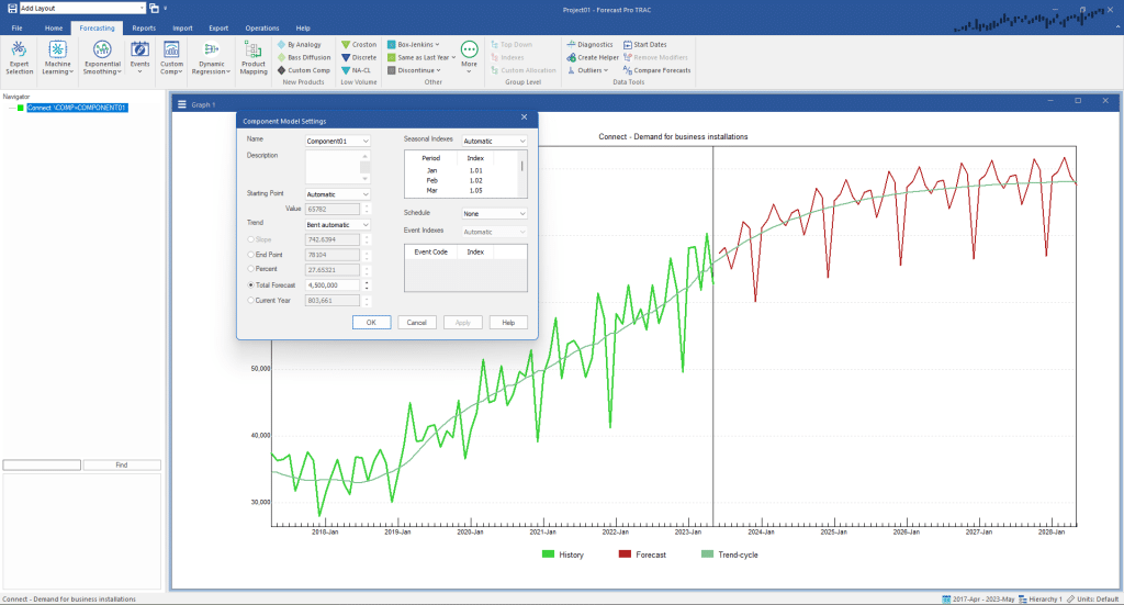
Now let’s explore using a bent trend. If you bend a trend downward, the monthly slope increment will decrease each forecast period resulting in a “bent” trend. If you bend a trend upward the monthly slope increment will increase each forecast period resulting in an exponential growth pattern.

There are two Bent trend options—automatic and custom. Bent automatic allows you to bend the automatically generated slope (which in our example was 742 units per month). Bent custom allows you to specify a custom slope and then bend it.

Use the Trend drop-down to select Bent automatic. Set Total Forecast to 4,500,000 and click the Apply button. Your screen should now match the one below.

Experiment with the Component Model Settings box including changing the Starting Point and Seasonal Indexes. Be sure to click the Apply button whenever you want to see the results from your current specification. When you are comfortable with the dialog box’s operation, exit Forecast Pro.