

When forecasting items that are similar, you may find that the same dynamic regression model specification works well across the different items. In this section, we will specify a price and promotion model for a specific market-level breakfast cereal Stock Keeping Unit (SKU) and then apply the same model specification to other breakfast cereal SKUs.
The data we will be using are weekly. Start the program, click the New Project icon and then click the Options icon. On the Basic tab, change the forecast horizon to 52 and click OK to close the Options dialog box. On the Home tab, click the Data Manager icon to open the Data Manager dialog. Click the Add drop-down on the Historic Data row, select Excel and select Cereal - Historic Data.xlsx to add it to the Historic Data row. Click the Add drop-down on the Explanatory Variables row, select Excel and select Cereal - Item Level Explanatory Variables.xlsx to add it to the Explanatory Variables row.
Click the Read & Forecast button to read in the historic demand data and click the Exit button to exit the Data Manager.
Right click on the Navigator to invoke its’ context menu and select Expand All to fully expand the Navigator. Select Cereal>C1 - Kids>Booth’s>BCT-013. Turn off the Override view by clicking the Overrides icon and click the Auto Arrange icon to maximize graph. Your display should now match the one shown below.
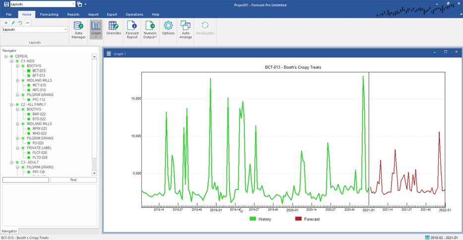
The data consists of weekly cereal sales for multiple sub-categories, brands and SKUs.
Forecast Pro allows you to specify two types of explanatory variables—global and item-specific. A global explanatory variable consists of a single time series (set of values) which can be included in a dynamic regression model for any item on the Navigator. An item-specific explanatory variable consists of a set of time series each of which is associated to a specific item on the Navigator.
To illustrate how this works, let’s consider our current example where we will be forecasting different cereal SKUs and using Price as an explanatory variable. If the price was the same across all SKUs we could define Price as a global explanatory variable. However, if the price varied by SKU we would want to define price as an item-specific explanatory variable to allow us input different prices for different SKUs.
In the electricity example we used global explanatory variables and you may have noticed that they were displayed in the Navigator. Because the values for item-specific explanatory variables are tied to specific items, they are not included on the Navigator.
In this example, we are using item-specific explanatory variables. Right click on the graph to bring up the graph context menu and select Settings. Click on the Add or Remove button to bring up the Add or Remove dialog box. On the filter drop-down, select Explanatory variables.
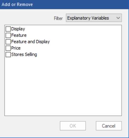
The Add or Remove dialog box now shows the five explanatory variables found in Cereal - Item Level Explanatory Variables.xlsx.
Display Percent of stores with item on display (e.g. End Cap), not featured in weekly ad circular
Feature Percent of stores with item featured in weekly ad circular
Feature and Display Percent of stores with item on feature and display
Price Average item price
Stores Selling The number of Stores selling the item
Select Price and click OK to return to the Graph Settings dialog box. Select the Relative Scaling box for price in the Graph Settings dialog box and press OK.
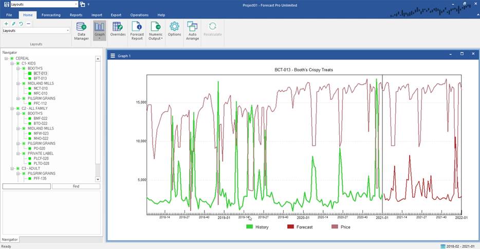
The graph now displays both weekly sales and price for Booth’s Crispy Treats. Notice that many of the sales peaks coincide with a decline in price.
In this example, explanatory variables have been defined for all items. Select Cereal on the Navigator and notice that Price is shown for total Cereal as well. Look at some of the other items in the Navigator as well. Notice that sales increase when price declines for most items.
Use the Graph Settings dialog box to explore the other explanatory variables. While you can display multiple explanatory variables simultaneously, it is usually easiest to observe the relationship between a given explanatory variable and sales if you look at a single explanatory variable at a time. Be sure to use the Relative Scaling checkbox so that you can clearly see if changes in the displayed explanatory variable correlate with sales increases or declines.
When you are done exploring the data, re-open the Graph Settings dialog box, turn off the explanatory variables and turn on the Fitted Values. Click OK to exit the dialog box and select Cereal>C1 - Kids>Booth’s>BCT-013. Your display should now match the one shown below.
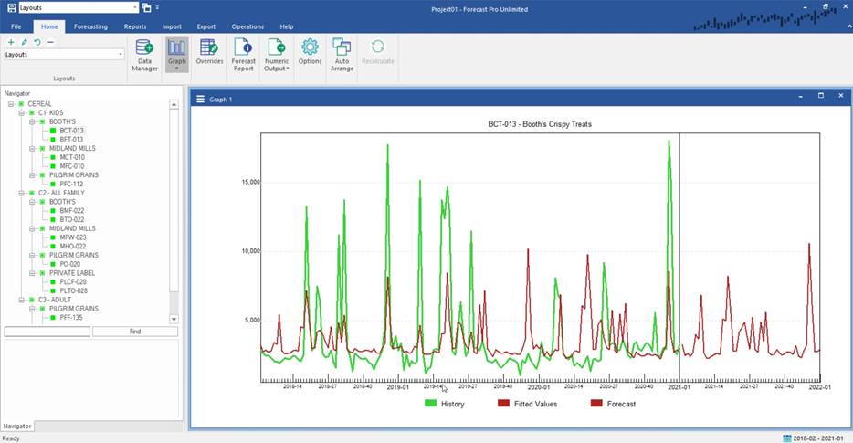
Open the Forecast Report by clicking the Forecast Report icon. Tile the display using the Auto Arrange icon. Scroll to the Within-Sample Statistics section of the Forecast Report and notice that the adjusted R-square for the expert selection model is 0.23.
We will now build a regression model for Booth’s Crispy Treats. Select the Forecasting tab. Price and Promotion models are often multiplicative. That is, changes in the explanatory variables drive percentage changes in the dependent variable. We build a multiplicative model by taking a log transform of the dependent variable and, optionally, non-negative explanatory variables. To build a multiplicative model, click the Custom Modifier icon in the Other group. In the Custom Modifier box, enter “Pow=Log” and click OK. This custom modifier instructs Forecast Pro to take the log of Cereal>C1 - Kids>Booth’s>BCT-013 before modeling it. Forecast Pro will reverse this transformation in the forecasts. We will show how to take log transforms of the explanatory variables below.
On the Forecasting tab, click the Dynamic Regression icon. In the Dynamic Regression dialog box, double click on each of the explanatory variables to add them to the model.
We will be using the model specification we build for Cereal>C1 - Kids>Booth’s>BCT-013 to forecast other SKUs, so let’s give this model specification a specific name. Click on the Name drop-down menu and select Save As. Enter “Price and Promotion” into the Save As dialog box and click OK.
Now let’s specify log transforms for our Price and Stores Selling explanatory variables. Right click on Price in the Model variable list box and select Transform>Logarithmic. Repeat this step for Stores Selling. The Dynamic Regression dialog box show look like below.
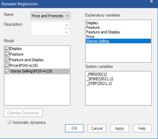
Click OK to apply the model and close the Dynamic Regression dialog box. Scroll down to the Within-Sample Statistics in the Forecast Report. Note that the adjusted R-squared has increased from 0.23 to 0.82, and the graph shows a much better fit. Scroll back up to show the regression coefficients.
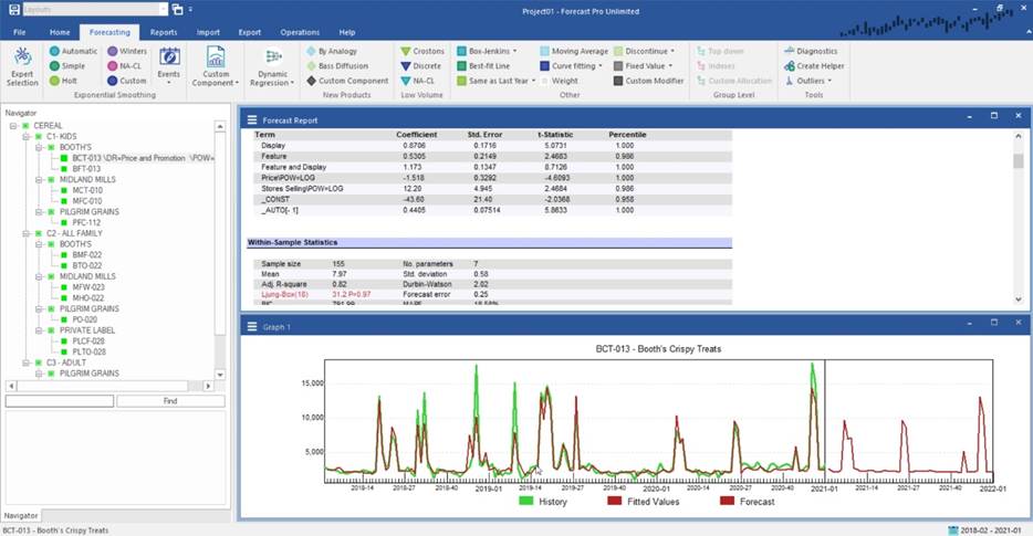
Note that all the explanatory variables are shown in black, meaning that they are significant, and the coefficients all have the expected sign, with features, displays and stores selling driving sales and price increases having a negative impact on sales.
Let’s apply this regression model to all items in the project. Right click on Cereal>C1 - Kids>Booth’s>BCT-013 to bring up the Navigator’s context menu and select Apply Modifier(s) To>This Level. We have now built price promotion models for all the end items.
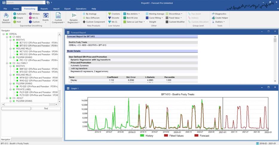
Click on a few end-items to view the different price and promotion models. Note that while the explanatory variables are the same in each model, the dynamic terms are customized to the end item. Select Cereal>C1 - Kids>Booth’s>BFT-013.
Exit Forecast Pro.
This concludes the Building Dynamic Regression Models lesson.